Full TFOP analysis
The full TFOP analysis with transit fitting carries out the steps required for ExoFOP submission and creates reduced light curves in fits-format that can be shared with collaborators. The main task of a multicolour transit candidate follow-up is to test whether the transit signal shows colour dependent variability in the transit depth (that is, the transit depth is chromatic), or whether the transit depth is same in all passbands (that is, the transit depth is achromatic).
The main steps for the full analysis are:
- Data appraisal: This is a fancy way of saying that we really need to have a look at the field and raw photometry before continuing anything else. It might be that all the necessary stars weren’t included into the photometry, or that the the photometry is useless because of weather, in which case we either need to redo the photometry of mark the observations as useless.
- Data cleanup: The photometry may be mostly good but contain outliers and strong systematics. These need to be cleared before continuing.
- Creation of the main TFOP output
- Plotting possible blends
- Plotting the covariates
- Saving the data in text tables
- Transit signal modelling
- Posterior optimisation
- Posterior estimation through MCMC sampling
- Light curve exporting The reduced photometry needs to be saved in fits format so that it can be easily used in subsequent analyses.
Field overview
After opening the notebook template you’ve created, you should see an example MuSCAT2 frame with apertures, sky annuli, and star IDs plotted together with a 2.5 arcmin circle centered around the target star (if the astrometry worked for the field). If you’re using a older version of the MuSCAT2 pipeline you’ll see just the full frame, but a newer version plots also a 5 and 2 arcmin-wide versions.
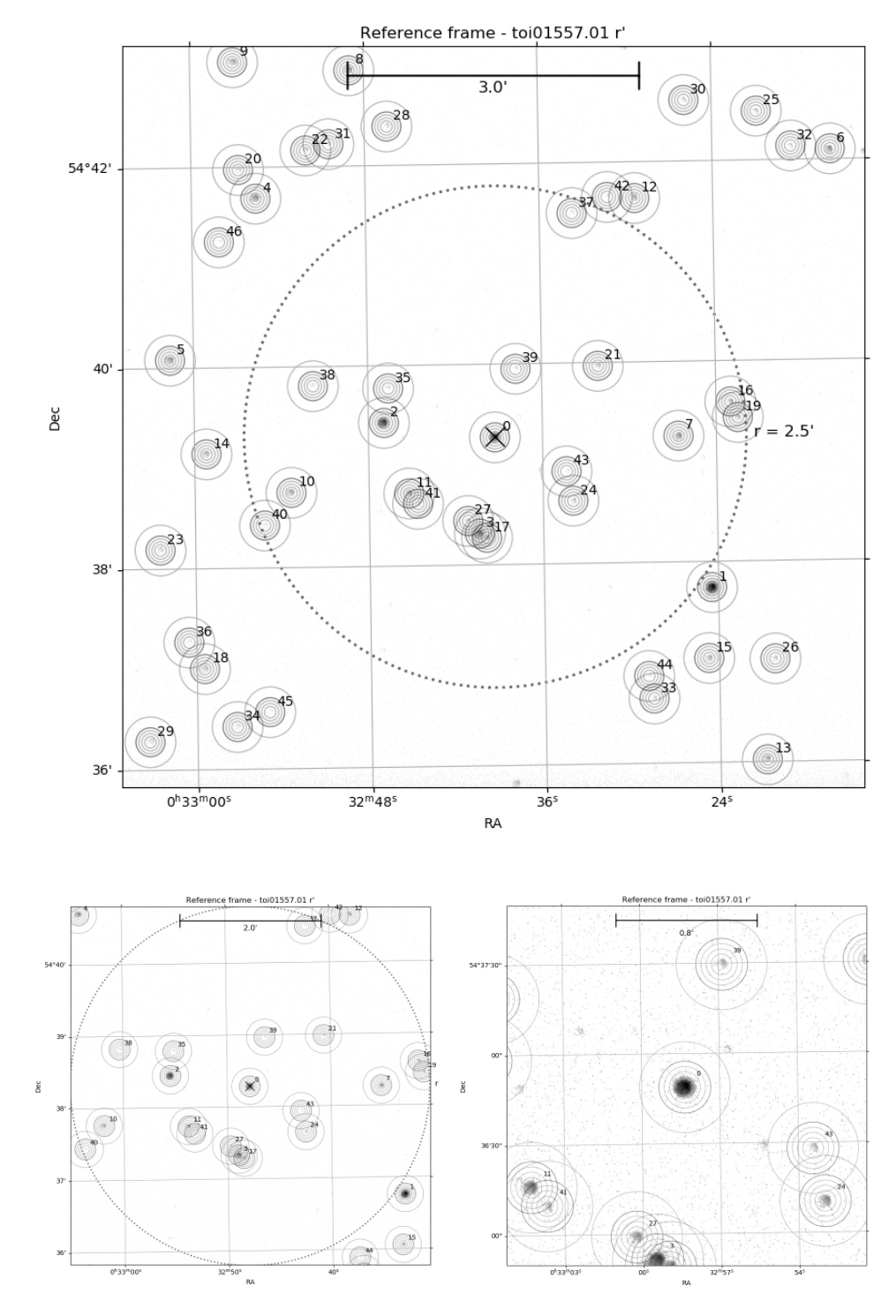
The concentric circles show the apertures used to calculate the photometry for each star. The apertures
are accessed by the aperture index (aid) that is 0 for the innermost aperture. The outermost aperture
can always be accessed as -1.
Before continuing, make sure that all the stars near the target star has been included into the photometry. That is, that all the black blobs are surrounded with apertures. If not, write to Hannu (or anyone else who knows how to run the photometry pipeline) that the photometry needs to be redone for the target.
TFOPAnalysis initialisation
The TFOP analysis is done with the muscat2ta.tfopanalysis.TFOPAnalysis class that contains all the necessary methods
for the TFOP data reduction and analysis.
TFOPAnalysis is initialised as
ta = TFOPAnalysis(TARGET, DATE, TID, CIDS)
where
TARGETis target name exactly as in the MuSCAT2 catalogDATEis the observing date in the formatyymmddTIDis the target ID. This should be 0 if we have an astrometric solution for the field, but can be something else if astrometry has failed for any reason. Please check the reference frames against the field shown for the target in the MuSCAT2 observation database.CIDSis a list of IDs of the useful comparison stars to include into the comparison star optimisation. Note: The final set of comparison stars will be a subset of these stars. The analysis is relatively robust against bad comparison stars, but each comparison star adds free parameters to the optimisation, so it’s best to constrain this to a small number of good comparison stars.
TFOPAnalysis has a set of optional arguments that can be used to fine-tune the analysis
passbands ['g','r','i','z_s']: passbands to include into the analysis.aperture_limits [(0, inf)]: a (min, max) tuple of aperture ID limits for the aperture optimisation.use_opencl [False]: use OpenCL (some parts of the computations will be done with the GPU) ifTrue.with_transit [True]: include a transit model into the light curve model ifTrue.contamination [None]: allow the flux to be contaminated by an unresolved star ifTrue.radius_ratio ['achromatic']:chromaticfor passband dependent radius ratios andachromaticfor passband independent radius ratios.npop [200]: number of parameter vectors in the optimisation and MCMC.toi [None]:TOIobject with the ExoFOP TOI information.
The pipeline prefills the TARGET, DATE, and TID arguments, but you’ll need to choose the comparison stars. The comparison
stars should be bright but not saturated, not blended with other stars of similar brightness, and without any intrinsic variability.
For example, analysis of TOI 1557.01 observed 19.8.2020 (the field shown above) would be initialised as
ta = TFOPAnalysis('toi01557.01', '200819', 0, [2,3,4])`
A warning is printed if the target or any of the comparison stars have saturated photometric points.
Light curve cleanup
Plotting raw light curves
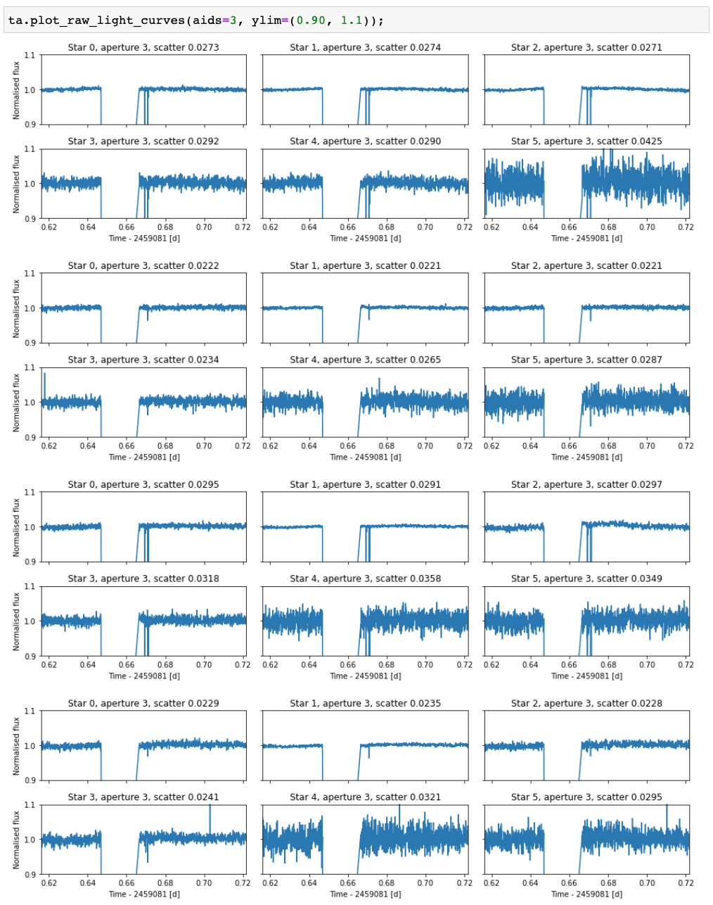
The first step is to look at the raw data, because this can already show any major issues with the observations (clouds, for example).
This is done with the TFOPAnalysis.plot_raw_light_curves method after the TFOPAnalysis has been initialised. By default, the
method plots the raw light curve for the target and five brightest stars for all passbands, but the plotted stars, apertures, and
everything else can be modified using the optional method arguments.
Cutting out sections of bad data
The raw light curves for our example case show that something weird happens around one thirds to the observations. All the fluxes drop
to zero for some time (could be a cloud or a dome failure), and we do not want to include this data to our analysis. We can use the
TFOPAnalysis.cut method to remove a section of the light curve
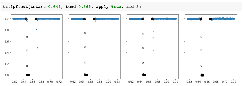
where the tstart and tend are given relative to the start of the night, as shown in the raw flux plot. We can also remove all
the points up to time t by setting tstart=-inf, tend=t, or all the points after time t by setting tstart=t, tend=inf.
The section to be removed can be visualised by setting apply=false, in which case the method creates a plot but does not touch
the data, and multiple sections can be removed from the data by calling the method multiple times with different parameters.
Outlier removal
Next, we can remove outliers using TFOPAnalysis.apply_normalised_limits (the method name may change soon…). The method fits a
polynomial to the normalised light curve and allows one to remove the points below a lower limit or above an upper limit.

Binning in time
Finally, we can bin the observations in time using the TFOPAnalysis.downsample method. While binning should be avoided in many
science cases, for TFOP analyses we can generally bin to 60 seconds without any loss in information.
ta.downsample(60)
Creating the ExoFOP output
Plotting possible blends
Checking the field for possible blended eclipsing binaries is one of the main tasks in ground-based photometric TESS follow-up. TESS pixels are large and it is common that many stars contribute to the photometry calculated over any aperture, and a signal identified as a transit can also be a faint eclipsing binary blended with a brighter star.
Plot the raw fluxes from all the stars that are within 2.5 arcmin from the target. The plot is saved to the final output directory.
These plots are important for TFOP and will be saved in the result directory. The plots show the raw light curves for the target star and all the stars around it within a given radius (unbinned and binned). The plots also show the expected times for the transit start, centre, and end (with their uncertainties), and the expected transit signal with depth corresponding to the depth that would be observed if the transit would be on the blending star (in reality we’d expect to see even deeper signal, because these plots assume blending only between the target and the possible blend, while in reality the blend is blended with multiple sources). The plots show the flux ratio between the target and the possible contaminant on the top-right corner.
ta.plot_possible_blends requires two arguments
- cid: comparison star index. Should be a bright (non-saturated) star outside a 2 arcmin radius of the target star.
- aid: aperture index. The aperture should be large enough to capture the flux of the brightest star within 2 arcmin from the target.
The possible blends are plotted using TFOPAnalysis.plot_possible_blends method:
ta.plot_possible_blends(cid=CID, aid=AID, caid=CAID)
where CID is a comparison star ID that should correspond to a bright (but not saturated) star outside of the 2 arcmin
circle, AID is the aperture index to use for the blending calculation, and CAID is the (optional) comparison star
aperture index that can be set if the comparison star is much brighter than the possible sources of blends.
Transit modelling
Wrapping up the analysis
The analysis is finished by calling the three TFOPAnalysis methods
ta.save()
ta.save_fits()
ta.finalize()
The first one saves the optimisation result and the MCMC samples, the second one saves the reduced light curves in fits format,
and the last one copies all the necessary files to the submit directory, including a partially filled report.txt file
that contains the final report that will be included into the ExoFOP submission.
After finishing the notebook, make sure you fill the report file. The analysis code prefills most of the required information, but not the final analysis conclusions. These should clearly state whether a transit signal occurs on the target and if the fitted transit signal shows significant chromatic variability. Also include any note you believe can be useful for people reading the report in ExoFOP and trying to decide if the observations show support for a planet transit or something else.